Mapping the Density States of a Superconductor as a Function of Energy
Summary
The Seamus Davis research group at the University of California
at Berkeley and at Cornell University, has performed research related
to the study of experimental condensed matter physics. Using a scanning
tunneling microscope, graduate student Kyle McElroy took an image
of a high temperature superconductor called Bi2Sr2CaCu2O8+x
and mapped the density of states of the superconductor as a function
of energy. In layman's terms, he made a map of the energy levels
of the electrons at different locations in the crystal.
 |
0.1

0 nm
|
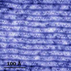
Fig 1: Atomic resolution image of the surface of the
high-temperature superconductor BSCCO. This image was acquired
with a sctunneling microscope. Each white dot is an
individual bismuth atom. The horizontal waves are an incommensurate
reconstruction due to stresses in the crystal.
|
Although a scanning tunneling microscope can map the
energy levels of the electrons as a function of position,
it cannot directly access the momentum of the electrons,
which is also very important for understanding the way the crystal
works. But with some pretty clever analysis, the momentum
information was backed out of the spatial information which
was acquired directly.
|
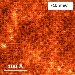
Fig 2: A map of the local electronic density of states
at energy -16 meV, in the same field of view as Fig 1. This
is effectively a density map of the number of electrons at
each spatial location which have energy -16 meV. There are
a number of different modulations and periodic structures
in several different directions: vertically and horizontally
and diagonally. Each of these modulations is an electron standing
wave.
|
0.8

0.18 nS
|
|
Details
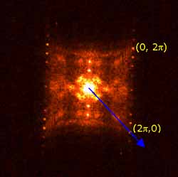
Another graduate student, Jenny Hoffman, took the
two dimensional Fourier Transform of the electron-density maps,
as a function of energy. The Fourier transform shows that there
are numerous modulations of the density of states, at multiple frequencies
and directions. There are too many modulations to see clearly by
eye in real space, but the different modulations are easily distinguished
in k-space.
These modulations are actually standing waves of electrons (an
electron is both a particle and a wave!). The exact wavevectors
of these standing waves were inverted to indicate the momentum of
the electrons. However, each k-space map has about sixteen 2-dimensional
peaks which had to be fit accurately, and Jenny had k-space maps
at dozens of energies. Unfortunately, much of the data was too noisy
for a 2-dimensional peak-fitting routine to converge reliably, so
the data had to be extracted in lines along all different angles
out from the zero-wavevector center of the k-space image, and then
the peaks in these lines had to be fitted. In fact, 16 peaks x 30
or more energies per dataset had to be analyzed! Once analyzed,
the parameter results from all fits had to be organized and used
to back out the crucial momentum information. This is where Origin
came in.
 |
0.6

0
nS Å
|
Fig 2: A map of the local electronic density of states
at energy -16 meV, in the same field of view as Fig 1. This
is effectively a density map of the number of electrons at
each spatial location which have energy -16 meV. There are
a number of different modulations and periodic structures
in several different directions: vertically and horizontally
and diagonally. Each of these modulations is an electron standing
wave.
|
Analysis in Origin
Jenny worked extensively with Origin C programming
to automate many aspects of her analysis in Origin. Functions were
created to assist her in importing the data, preparing the worksheet
for graphing and analysis, fitting the data, and visualizing the
data and results in graphical form. These functions were hooked
up to buttons placed on a custom worksheet template.

Fig 4: The buttons on the custom worksheet template.
Bringing in the data
An "Import" button was created and placed on the worksheet
template. The button uses LabTalk™ to bring up a dialog for
selecting the file to import. The script also calls an Origin C
function that handles the import once the file is selected. The
C function processes the data file, looking at and parsing header
information along the way, and then dumps the data into the worksheet
template.
Setting up the worksheet
A separate "Set XYXY" button was created to update the
worksheet column designations. This button also uses LabTalk script
to call an Origin C function.
Visualizing the data before analysis
The "Scatter Waterfall", "Line Waterfall",
and "LineSymb Waterfall" buttons were created to allow
you to plot the data as scatter, line, or line and symbol plots
prior to analysis. As with the other buttons, these three use LabTalk
to make calls to Origin C functions, which in turn perform the necessary
operations to plot the data and annotate the graph with information
from the selected columns of data.
Fitting the data
The analysis of the data took a lot of initial setup time, but
once this was completed, it was a snap. Jenny first created the
fitting functions to be used during the fitting process. She used
Origin's nonlinear curve fitter to do this.
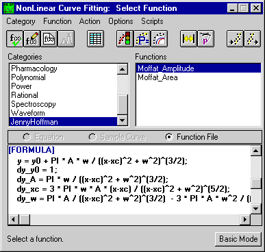 |
Fig 5: The Nonlinear Curve Fitter showing a fitting
function formula used in the analysis.
|
The fitting functions were then called from various Origin C functions
she created.
|
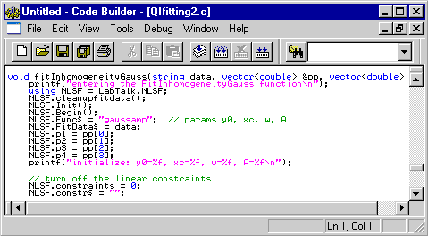
Fig 6: Origin's color-coded Code Builder interface
showing a portion of an Origin C function used to fit the
selected data.
|
|
The C functions were in turn called by the "Fit Selected"
button on the custom worksheet template.
// bring up attention box
break.style=1;
break.open("Loading and compiling Origin C function...");

// now attempt to load and compile function
if(run.LoadOC("%yOriginC\JEHprograms\JEHworkspace.ocw") != 0)
{
	// report if failure
	break.close();
	type -b "Error trying to load and compile the Origin C file.";
	break;
}
break.close();

//now call C function
prepareForFit(%H);
In addition, several worksheet and graph templates were utilized
during the fitting process. In all, the LabTalk script and Origin
C code behind the Fit Selected button was designed to automatically
perform the following operations:
- Fit all peaks automatically to a sum of several user-defined
functions
- Plot each fit on a graph template using the information from
the imported file (i.e. the file name and header information)
in order to label the axes
- Create an internal folder structure in the project to organize
each fit (specifically, put all the fits from a single energy
into a single folder)
- After all the fitting is done, plot each fit parameter as a
function of energy and plot one specific fit parameter as a function
of another
- Label all graphs correctly with information from the input file
names and headers
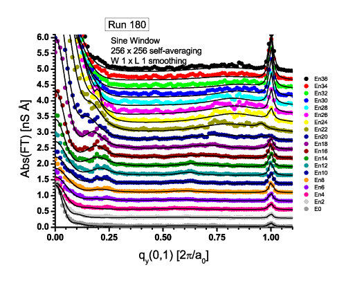
Fig 7: A final result graph including the raw data plotted
as scatter plots and the fit lines plotted as black line plots
Acknowledgements and Biographies
This work was performed in the research group of Seamus Davis,
a professor of physics at Cornell University who specializes in
experimental studies of condensed matter.
Kyle McElroy is a physics graduate student at the University of
California, Berkeley, currently working with Professor Davis at
Cornell University.
Dr. Jenny Hoffman
performed this analysis while she was a graduate student with Professor
Davis at the University of California at Berkeley. She is currently
a post-doc at Stanford University and will be starting as a professor
at Harvard University in January, 2005.
The scanning tunneling microscope used in this experiment was built
in the lab of Professor Davis by Dr. Shuheng Pan (now a professor
at the University of Houston) and Dr. Eric Hudson (now a professor
at Massachusetts Institute of Technology).
The BSCCO crystals used in this experiment were grown by Dr. Hiroshi
Eisaki (now at AIST-Tsukuba in Japan) and Professor Shin-ichi Uchida
at the University of Tokyo.
Parts of this work were funded by the New Energy and Industrial
Technology Development Organization of Japan, the Office of Naval
Research, Lawrence Berkeley National Laboratory, the National Science
Foundation, and Cornell University.